Tutorial

This tutorial contains a complete example that shows you how to use all the features of Syd. It will show you how to:

• Make a viewer with the factory method make_viewer() or by creating a subclass of Viewer.

• Add all the different types of parameters.

• Make hierarchical and inter-related callbacks.

• Get your data into the viewer.

0. Define a dataset for plotting.

Syd is designed to make it easy to explore data. For this tutorial, we’ll create a simple “dataset” that will show how you can reference data in your viewer. Since it’s a tutorial, it’ll be a bit contrived, but it’ll show you the principle of how to access data in a Syd viewer.

import numpy as np

# Create a simple dataset
T = 1000
amplitudes = list(np.linspace(1.0, 5.0, 100))
frequencies = list(np.linspace(1.0, 20.0, 100))
num_amplitudes = len(amplitudes)
num_frequencies = len(frequencies)

# Create a time array and an empty numpy array to store the data
t = np.linspace(0, 1, T)
data = np.zeros((num_amplitudes, num_frequencies, T))

# Fill the data array with the sine wave data
for i, amplitude in enumerate(amplitudes):
    for j, frequency in enumerate(frequencies):
        data[i, j, :] = np.sin(frequency * t * 2 * np.pi) * amplitude

# Create a dataset dictionary
dataset = {
    "amplitudes": amplitudes,
    "frequencies": frequencies,
    "t": t,
    "data": data,
}

# Now, we have a simple dataset to use. Let's pretend that it's a complicated and large dataset
# that you've stored on disk. You'll probably have a nice function that loads the data.
def load_data(amplitude, frequency):
    """Load the data for a given amplitude and frequency."""
    iamplitude = dataset["amplitudes"].index(amplitude)
    ifrequency = dataset["frequencies"].index(frequency)
    return dataset["t"], dataset["data"][iamplitude, ifrequency]

1. Create a viewer object.

As in the quickstart section, you will always start by making a viewer object. There are two ways to do this:

1. Factory-based Viewer (simple and flexible)

Use the make_viewer() function to instantiate an empty viewer object, then customize it by adding components programmatically.

2. Subclass-based Viewer (for advanced customization)

Subclass the Viewer base class to create an integrated viewer object for your specific use case. This approach is recommended when you need to encapsulate complex viewer behavior or reuse the same configuration across different contexts.

Factory-basedSubclass-based

# Start by importing the make_viewer function
from syd import make_viewer

# Then use it to make an empty viewer object!
viewer = make_viewer()

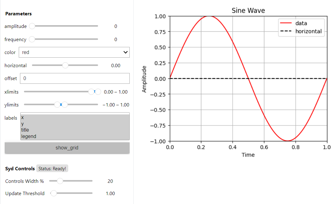
2. Add components to the viewer that will interactively control your plot.

Each component of Syd is associated with an “add_method” that should be used when you are building a new viewer. (For a reference to all the components, see Components.) When you create a new viewer, you should consider what parameters you need to control your plot, and then add the appropriate components to the viewer.

Each parameter has a set of attributes that you need to set when you add it to the viewer. For example, the add_integer method has the following attributes:

• name: The name of the parameter.

• min: The minimum value of the parameter.

• max: The maximum value of the parameter.

• value: The initial value of the parameter (only one not required).

For a full reference, see the Components page or the Viewer page.

In the dataset above, we have two parameters that we can control: the amplitude and the frequency. The dataset is composed of specific amplitudes and frequencies, so we can use an integer index to select which amplitude and frequency we want to plot.

Factory-basedSubclass-based

from syd import make_viewer

num_amplitudes = len(dataset["amplitudes"])
num_frequencies = len(dataset["frequencies"])

viewer = make_viewer()
viewer.add_integer("amplitude", min=0, max=num_amplitudes-1)
viewer.add_integer("frequency", min=0, max=num_frequencies-1)

Note

When you don’t specify a value for an integer (or a float or integer/float range), then it will be initialized to the minimum value (or (min, max) for a range).

Now, let’s say we also want to control a few other things about the plot:

Thing to control in the plot	How we’ll control it	Add method
The color of the plot	We’ll use a dropdown menu of color strings	add_selection()
A horizontal line indicating a particular value	We’ll use a float slider	add_float()
The vertical y-axis offset of the plot	We’ll use an unbounded float	add_unbounded_float()
The x-axis limits of the plot	We’ll use a float range slider	add_float_range()
The y-axis limits of the plot	We’ll use a float range slider	add_float_range()
Which labels to show	We’ll use a multi-select menu	add_multiple_selection()
Whether or not to show a grid	We’ll use a boolean checkbox	add_boolean()

Factory-basedSubclass-based

from syd import make_viewer

num_amplitudes = len(dataset["amplitudes"])
num_frequencies = len(dataset["frequencies"])

viewer = make_viewer()
viewer.add_integer("amplitude", min=0, max=num_amplitudes-1)
viewer.add_integer("frequency", min=0, max=num_frequencies-1)

# Add all the other components we want to control
viewer.add_selection("color", value="red", options=["red", "blue", "green"])
viewer.add_float("horizontal", value=0.0, min=-10.0, max=10.0)
viewer.add_unbounded_float("offset", value=0.0)
viewer.add_float_range("xlimits", value=(0.0, 1.0), min=-10.0, max=1.0)
viewer.add_float_range("ylimits", value=(-1.0, 1.0), min=-10, max=10)
viewer.add_multiple_selection("labels", value=["x", "y", "title", "legend"], options=["x", "y", "title", "legend"])
viewer.add_boolean("show_grid", value=True)

3. The state of the viewer

The state of the viewer is a dictionary that contains the current values of all the parameters in the viewer. You can access it by calling viewer.state (or self.state if you are using the subclass-based viewer).

The state is automatically updated whenever a parameter changes, and so reflects the current state of your GUI. Parameters (e.g. components) are always associated with a particular value, even at initialization. So, if you were to retrieve the state of the viewer right now, it would look like this:

Factory-basedSubclass-based

from syd import make_viewer

num_amplitudes = len(dataset["amplitudes"])
num_frequencies = len(dataset["frequencies"])

viewer = make_viewer()
viewer.add_integer("amplitude", min=0, max=num_amplitudes-1)
viewer.add_integer("frequency", min=0, max=num_frequencies-1)
viewer.add_selection("color", value="red", options=["red", "blue", "green"])
viewer.add_float("horizontal", value=0.0, min=-10.0, max=10.0)
viewer.add_unbounded_float("offset", value=0.0)
viewer.add_float_range("xlimits", value=(0.0, 1.0), min=-10.0, max=1.0)
viewer.add_float_range("ylimits", value=(-1.0, 1.0), min=-10, max=10)
viewer.add_multiple_selection("labels", value=["x", "y", "title", "legend"], options=["x", "y", "title", "legend"])
viewer.add_boolean("show_grid", value=True)

# You can access the current state of the viewer by calling viewer.state
print(viewer.state)
{
    "amplitude": 0,
    "frequency": 0,
    "color": "red",
    "horizontal": 0.0,
    "offset": 0.0,
    "xlimits": (0.0, 1.0),
    "ylimits": (-1.0, 1.0),
    "labels": ["x", "y", "title", "legend"],
    "show_grid": True,
}

4. The last figure generated by the Syd GUI

Similar to the state of the viewer, the last figure generated by the Syd GUI is stored in viewer.figure. If no figure has been generated yet, viewer.figure will be None. This is useful if you want to access the last figure – which is primarily for saving a figure without having to regenerate it. For the sub-class viewer, you can access it via self.figure instead of viewer.figure.

5. Adding buttons to your viewer

In addition to parameters, you can also add buttons to your viewer to perform actions. The most common use case for a button is to save the current figure – but of course many things are possible!

Buttons are added using the add_button() method. This method has the following attributes:

• name: The name of the button.

• label: The label of the button.

• callback: The function to call when the button is clicked. (See the 7. Adding callbacks to the viewer. section for more details.)

• replot: Whether to replot the figure when the button is clicked.

You can also update buttons in a similar way to parameters (with the update_button() method).

Note

Consider whether to set replot=False carefully! If you set it to False, the figure will not be updated after you click the button… even if clicking the button causes changes to other parameters! The parameters will be changed, but the plot won’t regenerate until you change a parameter.

Let’s add a button to our viewer that will save the current figure. The callback function will be save_figure, which will save the current figure to a file called figure.png. Again – see the 7. Adding callbacks to the viewer. section for more details on how callbacks work. Note how we use the viewer.figure / self.figure attribute to get the current figure.

Factory-basedSubclass-based

from syd import make_viewer

num_amplitudes = len(dataset["amplitudes"])
num_frequencies = len(dataset["frequencies"])

viewer = make_viewer()

def save_figure(state):
    # Get the current figure
    fig = viewer.figure

    # Save the figure
    fig.savefig("figure.png")

# Note: the save_figure function is defined after the viewer is created so the
# reference to viewer.figure is clearly defined. For best practice, use a subclass
# based viewer to make sure that self.figure is the figure you're looking for!

viewer.add_integer("amplitude", min=0, max=num_amplitudes-1)
viewer.add_integer("frequency", min=0, max=num_frequencies-1)
viewer.add_selection("color", value="red", options=["red", "blue", "green"])
viewer.add_float("horizontal", value=0.0, min=-10.0, max=10.0)
viewer.add_unbounded_float("offset", value=0.0)
viewer.add_float_range("xlimits", value=(0.0, 1.0), min=-10.0, max=1.0)
viewer.add_float_range("ylimits", value=(-1.0, 1.0), min=-10, max=10)
viewer.add_multiple_selection("labels", value=["x", "y", "title", "legend"], options=["x", "y", "title", "legend"])
viewer.add_boolean("show_grid", value=True)
viewer.add_button("save_figure", label="Save Figure", callback=save_figure, replot=False)

6. Add a plot method to the viewer.

The plot method is the most important method in a viewer. It is called whenever the viewer’s state changes, and it is where you update the plot based on the current state.

There are some key rules about the plot method:

Important

Plot methods should accept a single argument, which is the current state of the viewer.

# For factory-based viewers, the signature should look like this:
def plot(state):

# For subclass-based viewers, the signature should look like this:
class YourViewer(Viewer):
    def plot(self, state):

Important

Plot methods should create and return a matplotlib figure.

def plot(state):
    # Make a new figure in your plot function
    fig = plt.figure()
    # ... do some stuff to make your plot ...

    # Then return the figure object!!!!
    return fig

Important

Plot methods should not call plt.show()!

Syd will handle displaying the figure for you. Calling plt.show() will cause your plot to be displayed twice and other unexpected behavior.

Let’s make our plot method!

Factory-basedSubclass-based

from syd import make_viewer

viewer = make_viewer()

# ... all the add_* methods ...
# ... adding the save_figure functionality ...
def plot(state):
    # Get the data based on the current state
    current_amplitude = dataset["amplitudes"][state["amplitude"]]
    current_frequency = dataset["frequencies"][state["frequency"]]
    time, data = load_data(current_amplitude, current_frequency)

    # Get all the other parameters for plotting
    color = state["color"]
    horizontal = state["horizontal"]
    offset = state["offset"]
    xlimits = state["xlimits"]
    ylimits = state["ylimits"]
    labels = state["labels"]
    show_grid = state["show_grid"]

    # Make your figure
    fig, ax = plt.subplots(1, 1, figsize=(5, 4), layout="constrained")
    ax.plot(time, data + offset, color=color, label="data")
    ax.axhline(horizontal, color="black", linestyle="--", label="horizontal")
    ax.set_xlim(xlimits)
    ax.set_ylim(ylimits)
    if "x" in labels:
        ax.set_xlabel("Time")
    if "y" in labels:
        ax.set_ylabel("Amplitude")
    if "title" in labels:
        ax.set_title("Sine Wave")
    if "legend" in labels:
        ax.legend(loc="best")
    if show_grid:
        ax.grid()

    # Return the figure
    # ~ WITHOUT CALLING plt.show()!!! ~
    return fig

# Tell the viewer to use your plot method
viewer.set_plot(plot)

# Note: if the plot method existed already, you could have done this:
# viewer = make_viewer(plot)

7. Adding callbacks to the viewer.

A callback is a function that is called in response to some event. Syd enables you to implement callbacks with the on_change() method.

Important

1. You define a callback function that should be called whenever certain parameters change.

2. You add that callback function to your viewer and tell Syd which parameters should initiate a call to it.

3. Callback functions follow the same rules as the plot method.

   Factory-based viewers should have a signature like your_callback(state)

   Subclass-based viewers should have a signature like your_callback(self, state)

4. To change parameters during a callback, use the update_* methods!

   There is an update method associated with each parameter type (it has an identical API to the add methods…). For more info on this, check out the Components section.

Let’s think about what callbacks this viewer might need.

• We added a mechanism to add an unbounded offset to the data!

• This means that the y-values of the data can be anything.

• But, the horizontal line and the y-limits have specified min/max values, which might not overlap with our data.

• So, we’ll need a callback that changes the range of the horizontal line and the y-limits to be the same as the data.

• This will need to be changed whenever the amplitude or offset is updated.

Factory-basedSubclass-based

from syd import make_viewer

viewer = make_viewer()

# ... all the add_* methods ...
# ... adding the save_figure functionality ...
# ... adding the plot method ...

# Create a callback function that accepts "state" as an argument
def update_offset(state):
    # Get the data based on the current state
    current_amplitude = dataset["amplitudes"][state["amplitude"]]
    current_frequency = dataset["frequencies"][state["frequency"]]
    data = load_data(current_amplitude, current_frequency)[1]

    # Get the offset
    offset = state["offset"]
    min_plot_data = np.min(data + offset)
    max_plot_data = np.max(data + offset)

    # Update the min/max values of the horizontal line and the y-limits to match the plot data
    viewer.update_float_range(
        "ylimits",
        value=(min_plot_data, max_plot_data),
        min=min_plot_data,
        max=max_plot_data
    )
    viewer.update_float("horizontal", value=offset, min=min_plot_data, max=max_plot_data)

# Add the callback to the viewer
# The syntax here is:
# viewer.on_change("parameter_name", callback_function)
# Or if multiple parameters require the same callback, you can do this:
# viewer.on_change(["parameter_name_1", "parameter_name_2"], callback_function)
viewer.on_change(["amplitude", "offset"], update_offset)

Note

For more examples on callbacks, check out the hierarchical callbacks example or run it yourself in colab:

8. Show or share the viewer!

And that’s it! You’ve made an advanced Syd viewer that can load data, plot it, and update it interactively.

The next step is to show or share the viewer. Syd is designed to seamlessly work in both jupyter notebooks and web browsers. To see your viewer in a notebook, you can use the show() method. To see your viewer in a web browser, you can use the share() method. Both have different benefits. The notebook version is great for quickly exploring your data locally. The browser version is fast and quick too, with a slightly different style, and is awesome for sharing with others on your local network (it’s hosted at your computers IP address, so you can send a link to your PI and have them open it on their computer!).

NotebookBrowser

viewer.show() # for viewing in a jupyter notebook

9. Putting it all together!

Now that we have gone through all the steps, let’s put it all together in a single place.

Both the factory-based and subclass-based examples are shown below in full, and in addition, if you want to see them in action, you can check out the examples in a notebook or on colab:

Factory-basedSubclass-based

Check out the full factory example in a notebook, or run it yourself in colab:

import numpy as np
from matplotlib import pyplot as plt
from syd import make_viewer

# Create a simple dataset
T = 1000
amplitudes = list(np.linspace(1, 5.0, 100))
frequencies = list(np.linspace(1, 20.0, 100))
num_amplitudes = len(amplitudes)
num_frequencies = len(frequencies)

# Create a time array and an empty numpy array to store the data
t = np.linspace(0, 1, T)
data = np.zeros((num_amplitudes, num_frequencies, T))

# Fill the data array with the sine wave data
for i, amplitude in enumerate(amplitudes):
    for j, frequency in enumerate(frequencies):
        data[i, j, :] = np.sin(frequency * t * 2 * np.pi) * amplitude

# Create a dataset dictionary
dataset = {
    "amplitudes": amplitudes,
    "frequencies": frequencies,
    "t": t,
    "data": data,
}

# Now, we have a simple dataset to use. Let's pretend that it's a complicated and large dataset
# that you've stored on disk. You'll probably have a nice function that loads the data.
def load_data(amplitude, frequency):
    """Load the data for a given amplitude and frequency."""
    iamplitude = dataset["amplitudes"].index(amplitude)
    ifrequency = dataset["frequencies"].index(frequency)
    return dataset["t"], dataset["data"][iamplitude, ifrequency]

num_amplitudes = len(dataset["amplitudes"])
num_frequencies = len(dataset["frequencies"])

# Make the viewer and add all the components
viewer = make_viewer()

def save_figure(state):
    """After viewer is created for clear reference"""
    figure = viewer.figure
    figure.savefig("figure.png")

viewer.add_integer("amplitude", min=0, max=num_amplitudes-1)
viewer.add_integer("frequency", min=0, max=num_frequencies-1)
viewer.add_selection("color", value="red", options=["red", "blue", "green"])
viewer.add_float("horizontal", value=0.0, min=-10.0, max=10.0)
viewer.add_unbounded_float("offset", value=0.0)
viewer.add_float_range("xlimits", value=(0.0, 1.0), min=-10.0, max=1.0)
viewer.add_float_range("ylimits", value=(-1, 1), min=-10, max=10)
viewer.add_multiple_selection("labels", value=["x", "y", "title", "legend"], options=["x", "y", "title", "legend"])
viewer.add_boolean("show_grid", value=True)
viewer.add_button("save_figure", label="Save Figure", callback=save_figure, replot=False)

def plot(state):
    # Get the data based on the current state
    current_amplitude = dataset["amplitudes"][state["amplitude"]]
    current_frequency = dataset["frequencies"][state["frequency"]]
    time, data = load_data(current_amplitude, current_frequency)

    # Get all the other parameters for plotting
    color = state["color"]
    horizontal = state["horizontal"]
    offset = state["offset"]
    xlimits = state["xlimits"]
    ylimits = state["ylimits"]
    labels = state["labels"]
    show_grid = state["show_grid"]

    # Make your figure
    fig, ax = plt.subplots(1, 1, figsize=(5, 4), layout="constrained")
    ax.plot(time, data + offset, color=color, label="data")
    ax.axhline(horizontal, color="black", linestyle="--", label="horizontal")
    ax.set_xlim(xlimits)
    ax.set_ylim(ylimits)
    if "x" in labels:
        ax.set_xlabel("Time")
    if "y" in labels:
        ax.set_ylabel("Amplitude")
    if "title" in labels:
        ax.set_title("Sine Wave")
    if "legend" in labels:
        ax.legend(loc="best")
    if show_grid:
        ax.grid()
    return fig

# Tell the viewer to use your plot method
viewer.set_plot(plot)

# Create a callback function to change the y-limits and horizontal line based on the offset
def update_offset(state):
    # Get the data based on the current state
    current_amplitude = dataset["amplitudes"][state["amplitude"]]
    current_frequency = dataset["frequencies"][state["frequency"]]
    data = load_data(current_amplitude, current_frequency)[1]

    # Get the offset
    offset = state["offset"]
    min_plot_data = np.min(data + offset)
    max_plot_data = np.max(data + offset)

    # Update the min/max values of the horizontal line and the y-limits to match the plot data
    viewer.update_float_range("ylimits", value=(min_plot_data, max_plot_data), min=min_plot_data, max=max_plot_data)
    viewer.update_float("horizontal", value=offset, min=min_plot_data, max=max_plot_data)

# Add the callback to the viewer
viewer.on_change(["amplitude", "offset"], update_offset)

# Show the viewer!
viewer.show() # for viewing in a jupyter notebook
# viewer.share() # for viewing in a web browser